
This March, we’re going BIG.
I’ve been trying to master the art of the perfect bracket since the 2013 tournament. I’m one of those guys that maxes out his 10 ESPN brackets, his 3 CBS brackets, and however many brackets Yahoo allows. He only did it one year, but I’ve spent the $1 billion from Warren Buffett’s bracket challenge in my head many times over (I’m starting a charitable foundation, obviously). One year I managed to get one of my ESPN brackets in the top 99.98 percentile on the site, but that was probably due more to sheer volume than skill.
Still, the hunt continues for perfection, and this year I’m bringing more data-driven tools than ever before. And yes, I built all of these tools myself in the statistical programming language R. I imported nothing other than official NCAA stats for teams and players. The outputs exist in a series of .csv files that are connected by a large Excel spreadsheet. I am working to build an interface that will make all or part of my work public, but that’s still a work in progress for now. For now, we’ll be posting analyses of first-round matchups and team profiles after the bracket is announced.
So without further ado, here’s what we’ve got in the Fayette Villains toolbox.
The Checklist
Anyone giving you bracket advice will probably tell you not to try and pick all the upsets and instead focus on getting as many of the Final Four or Elite 8 correct as possible. That’s great advice if you’re wanting to win your office pool, but it’s terrible advice if you’re a perfectionist like me whose bracket is usually in the trash can after the first weekend. My focus is on the first round. I want to go 32-0. I’ve gotten fairly close before (28-4 is my best, I think).
To do that, I’m focusing most of my effort on the first-round matchups. I’m creating 32 checklists, one for each game. I’ll run each game through each of my tools, then mark the team favored by each tool. That will give me a comprehensive view of the game so I can make a decision.
It would be too involved to do the full checklist thing for games after the first round, but I’ll still use these tools to pick the rest of the bracket.
Note: Am I serious with this? You may wonder as you read it. Here’s my answer: no, I do not actually expect to make a perfect bracket with these tools. I do this for fun. Yes, this is fun for me, and yes, these are serious tools of data science. I hope it is fun for you to read about it.
#1 Traditional Model
The Traditional Model picks the score of each game. It’s at 51% against the spread so far this season with 3,357 games picked as of February 27th. It works in a manner similar to KenPom’s ratings: each team has an Adjusted Offensive Efficiency, Adjusted Defensive Efficiency, and Adjusted Scoring Margin. As of this writing, for example, Arkansas’ AOE is 105.6 (Arkansas would score 105.6 points per 100 possessions against an average defense), its ADE is 90.4 (Arkansas would allow 90.4 points per 100 possessions against an average offense), and its ASM — the difference between AOE and ADE — is +15.1 (Arkansas would beat an average D-1 team by 15.1 points in a 100-possession game). These ratings are calculated using team stats adjusted for quality of opponent and updated daily.
In order to use the traditional model to pick scores, we need only determine how many possessions will be in the game and go from there. I use average possession length to make that determination: if Arkansas’ offense averages 16.3 seconds per offensive possession and its opponent averages 17.8 for theirs, then we can assume that 34.1 seconds will pass, on average, for each team to record one possession. Over a 40-minute game, that comes out to 70.4 possessions. (It’s actually slightly more complicated, as Arkansas’ 16.3 seconds APL has to be adjusted for how fast the defense usually allows offenses to play, but you get the gist.)
Now can adjust the per-100-possession numbers to get a score. Arkansas’ score would be as follows:
Arkansas Score = ( Arkansas AOE – ( Average ADE – Opponent ADE ) ) * (Possessions / 100)
Arkansas’ AOE is adjusted downward based on the quality of the defense, and then the whole thing is adjusted by the expected number of possessions.
This model is very good at accounting for quality of opponent, but does little to account for the specific matchup. For that, we need a different model.
#2 Matchup Model
The matchup model comes from a Ken Pomeroy study on who has “control” of certain stats, the offense or the defense. As an easy example, free throw percentage is very clearly under the offense’s control. The defense cannot influence it. But other stats, like 2-point percentage, offensive rebounding percentage, and many others, are “up for grabs”, you might say. Pomeroy found that variations in 2-point percentage are due about 50% to the offense and 50% to the defense. Steals are about 70% under the defense’s control, while 3-point rate is about 70% under the offense’s control.
We can use those “control” weights and component stats to assemble an entire box score. Here’s an example from the code that executes this model:

The highlighted portion is how the model picks the home team’s 3-point percentage. KenPom found that 3-point percentage is 80% under the offense’s control, or 4:1, to use a ratio. So the home team’s base 3-point percentage distance from the mean is modified by 1, while the away team’s base 3-point defense distance from the mean is modified by 0.25, as it only has one-fourth the influence of the offense.
Through 3,357 games picked this year, the matchup model is about 52% against the spread. We use it in our “Place Your Bets” pieces. It is great at factoring in matchups while still giving a score prediction. Its primary weakness is that it does not do much to account for the quality of competition, which means mid-majors that dominated one-bid leagues will be overrated by this model because of their inflated stats. Still, it’s having a good year.
#3 Performance Trends
Ultimately, picking the score alone isn’t the only way to go. We have to look at more open-ended factors. Momentum is a big one. A team that dominated November and December but has played poorly of late may be overrated by models that use all-season stats. What have you done for me lately?
Our analysis of performance trends involves game scores, which are just normalized AOE and ADE values from each game. For example, Arkansas’ raw offensive efficiency was 109 against Kentucky, but due to the quality of Kentucky’s defense, it became 124 adjusted offensive efficiency. An AOE of 124 is in the 86th percentile of all offensive performances this season, so the Hogs got an offensive game score of 86. Make sense? Perfect. Game score will be used in several of these tools.
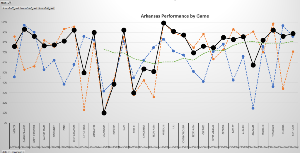
In this graph of trended game scores (through the UK game), we can see Arkansas’ season in a nutshell. You can clearly see the ugly stretch of 5 losses in 6 games, the 100 game score in the 87-43 win over Mizzou, and the strong basketball since then. The blue line is offense and the orange line is defense, while the black line is overall.
The green line is where things get interesting. That’s a running 10-game average overall game score. We can use it to see who is playing well at the right time.
Game score is very useful because it tells us how well a team spreads out their good stats. Are they highly ranked in AOE because they had one or two amazing performances and a bunch of mediocre ones? Are they highly ranked because their offense was amazing months ago, and their stats are still reaping the benefits? Or are they consistently strong and/or peaking in March?
#4 Matchup Analysis
This is a more open-ended version of the matchup model. There’s no score prediction at the end, just the “my offense versus your defense” stats laid bare on a table for easy comparison. Here’s an example:
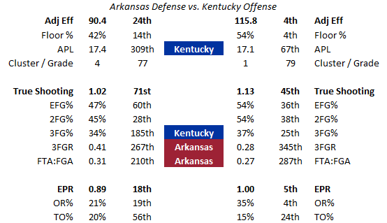
This is Arkansas’ defense matched up with Kentucky’s offense. Right off the bat, we see that Arkansas has an advantage in terms of free throw rate (the Hogs ended up with just 4 second-half fouls in the game). Kentucky has an advantage in terms of pace (sure enough, the Cats gave Arkansas problems when they were able to run on offense). But it is mostly an even matchup, as you can see.
Matchup tables like these are useful because you can easily gauge how a team will be able to build on its strengths and manage its weaknesses, given the matchup. These tables are also used in conjunction with the next two tools.
#5 Cluster Analysis
In statistics and data science, a “cluster” is a group of data points. K-means clustering is an unsupervised learning tool that takes a bunch of data points and groups them according to their similarities. In this case, those data points are teams, and “their similarities” (or differences) are all of their season statistics.
The value of clustering is obvious. You’ve probably heard talking heads say things like “Team X struggles against good rebounding teams, and their next opponent is great at crashing the boards.” K-means clustering allows us to qualify statements like that.
All 358 Division I teams get placed into an offensive cluster and a defensive cluster. Here’s how I performed my cluster analysis (done twice, once for offense and once for defense):
- An initial k-means clustering function is run on a table of data that includes every team and every single raw statistic I have on them. A k-selection test shows we need 4 offensive clusters and 5 defensive clusters.
- An ANOVA model is run on the results to find which individual statistics influenced the data the most. Not every statistic is actually relevant: free throw percentage, for instance, isn’t useful for defining clusters. The ANOVA results pointed to four stats for offensive clusters: true shooting, 3-point rate, offensive rebounding, and pace. That makes logical sense: KenPom found that 3-point rate and pace are largely under the offense’s control, and how well teams shoot and rebound is indicative of their scheme. The four defensive stats are these: true shooting, floor percentage, free throw rate, and EPR. This also makes sense (free throw rate is one of the few statistics that the defense mostly controls). Floor percentage has some issues because it is colinear with the others (colinearity refers to how variables influence each other) but I used it anyway.
- The k-means clustering model is re-run with the 4 stats for each side of the ball. Each team is assigned an offensive and defensive cluster number.
- The average game score against each cluster is referenced and placed in a table. For example, Arkansas has an average offensive game score against each of the 5 defensive clusters, and vice versa.
Here is how the clusters are used in the matchup analysis:
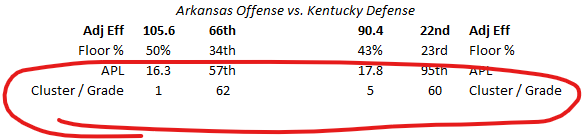
This table tells us that Arkansas’ offense is in offensive cluster 1 and Kentucky’s defense is in defensive cluster 5. Arkansas has an average offensive game score of 62 against cluster 5 defenses, while Kentucky has an average defensive game score of 60 against cluster 1 offenses.
This actually proved to be relevant in the game: Kentucky’s 60 against cluster 1 is its worst among the 4 offensive clusters. Sure enough, the Wildcat defense struggled with Arkansas’ offense, posting a defensive game score of 45, its second-worst of the season. Cluster analysis tells us how a team usually performs against opponents similar to what they’ll be facing.
#6 Correlation Matrix
I was introduced to the value of correlation matrices in 2018. After UMBC upset Virginia in the first-ever 16-over-1 upset, someone posted a chart on Twitter that showed that for UMBC, opponents making 3-pointers was highly correlated with UMBC losing. But for Virginia, even attempting 3-pointers on offense was correlated with the Cavaliers losing. So Virginia could not exploit UMBC’s biggest weakness without risking their own.
Now, there were some problems with that claim. “Correlated with losing” is doing a lot of work here: Virginia had lost only one game all season, so we had a sample size issue. So I decided to build a correlation matrix for each team that, instead of correlating with win/loss, was correlated with game scores. So stats like “3-pointer made” is correlated with offensive game score.
A bunch of different stats go into the correlation matrix: free throw missed, opponent 2-point attempt, unassisted field goal made, shot opportunity by an opposing power forward or center. All pulled straight from each game’s box score. Here’s an early prototype for the Hogs (I’m planning add more stats to the final version):
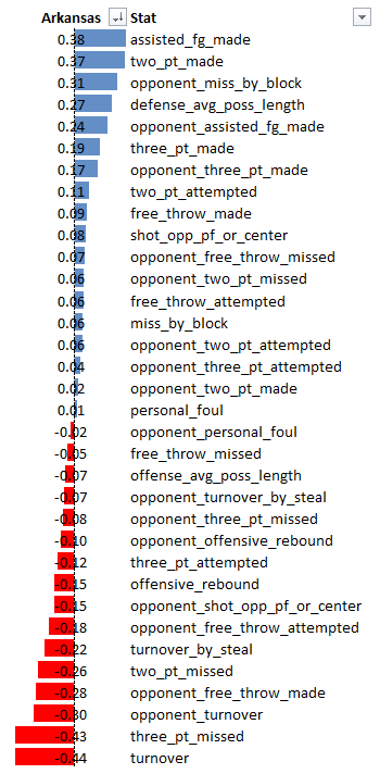
The number one stat for Arkansas is turnovers by the offense, with a correlation of -0.44 to offensive game score. Missed 3-pointers, made 2-pointers, assists, blocked shots, and defensive pace (!) are also major factors. That last one could be very interesting depending on the matchup.
Correlation matrices have obvious value: they tell you what a team needs to do to play well. When a team is at their best defensively, what are they doing well? Are they forcing more turnovers than usual? Fouling less than usual? Defending the perimeter better than usual? Once we have the correlation tables, we can look at the matchup tables and see if the matchup is favorable for the highest-priority stats.
#7 Decision Tree / Random Forest / Neural Net
Okay, so I’ve saved the worst for last. Not exactly going out with a bang. I want this one to provide value, but I’ve been working on it for years, and so far, it’s just not super accurate.
The idea for this came with the first NCAA Tournament I went all-in to predict: 2013. I noticed that most of the Cinderellas that pulled first-round upsets had things in common: namely, they played at a fast pace and shot well from 2. Their victims also all played at a slow pace. I wondered if low seeds that pull upsets have some things in common, or if teams that get upset have things in common.
Decision trees (and random forests, their more thorough and complicated cousins) are somewhat similar to correlation matrices: they look at a bunch of input stats and see if there’s a pattern with the game result. This year’s models are my biggest yet: six years of first-round NCAA Tournament results, a total of 192 games, with that-season team stats for all 384 teams involved. Each line of data given to the model has the stats for both teams and a result to look for: Favorite or Underdog. The model establishes a set of rules that can visualized like branches on a tree (hence the name), or a choose-your-own-adventure book. Maybe one branch groups all data points where the favorite shoots less than 33% from 3 in one node and more than 33% in another. These rules are established based on patterns the model finds, and branching continues in hopes of finding a clear result.
Neural nets work similarly but are much more complicated and more difficult to understand. Rather than return a single pick, a neural net will return a continuous value from 0 to 1, so it may say a game has a 63% chance of ending in an upset based on how its stats aligned with the previous data that was fed into the model.
Previous decision trees I’ve built have managed to call a few upsets, but they just are not very accurate overall, and I’m still hesitant after one I built a few years back called for Stony Brook to beat Kentucky and they lost by 30. I haven’t built this year’s yet, but it will be the biggest of all, so maybe the larger sample size will help it out.
Conclusion
So, those are the tools! As I said above, for each matchup I put notes next to each of the seven tools and take a final comprehensive look before picking the game. I try to identify games where I’m 100% confident in the outcome, so I can pick those in every bracket I fill out. That leaves a little wiggle room for games I’m unsure of, so I can pick one result in one bracket and another result in a different bracket.
Keep an eye on this space after the bracket reveal. I’ll be posting pieces of analysis from my look at the first-round matchups to use in filling out your own bracket. If my advice ends up being horribly wrong and ruins your bracket, don’t blame me: I’m just having fun here.